LIDAR Wizard Overview
The wizard is accessed from the Tool Strip and is only accessible when the Project Map is active. The primary purpose of the LIDAR wizard is to use the boundary area to quickly find, download, clip, and process public LIDAR tiles. The wizard searches the indexed tiles to find available USGS LIDAR tiles and provides options for download. Downloaded LIDAR in LAS or LAZ format can be processed in one step to generate a single DEM with hillshade image, dxf contours and a 3D View. Output is copied to a Jobs folder for easy access and incorporation to your primary CAD or GIS workflow. The basic wizard process:
-
Select the source boundary – created from the map. When you select the boundary layer the US state the boundary is contained in is identified. If the state shown is incorrect, then pick the US State you want to use for searching.
-
Click the Find Button to search – using the selected state and the selected boundary layer the application searches for available LIDAR sources. More than 1 source may be returned in the tree list. The search always returns USGS Quick Terrain (Web) as a source. USGS Quick Terrain (Web) queries best terrain data from the USGS 3DEP web services for the area and attempts to colorize using an image from the USGS NAIP Web service. The USGS Quick Terrain (Web) query is limited to a width of 2000 pixels so the returned point grid size will be approximately the width of the boundary layer extents divided by 2000 in map units.
-
Select an Elevation Source – from the tree list select an item.
- USGS Quick Terrain: (Make sure you set the Projection to match your target output.) The application will query the USGS 3DEP web service and the USGS NAIP web service and download a point cloud clipped to the bounding box of the boundary layer. The download process will warp the point cloud to match the specified Coordinate Reference System (Projection).
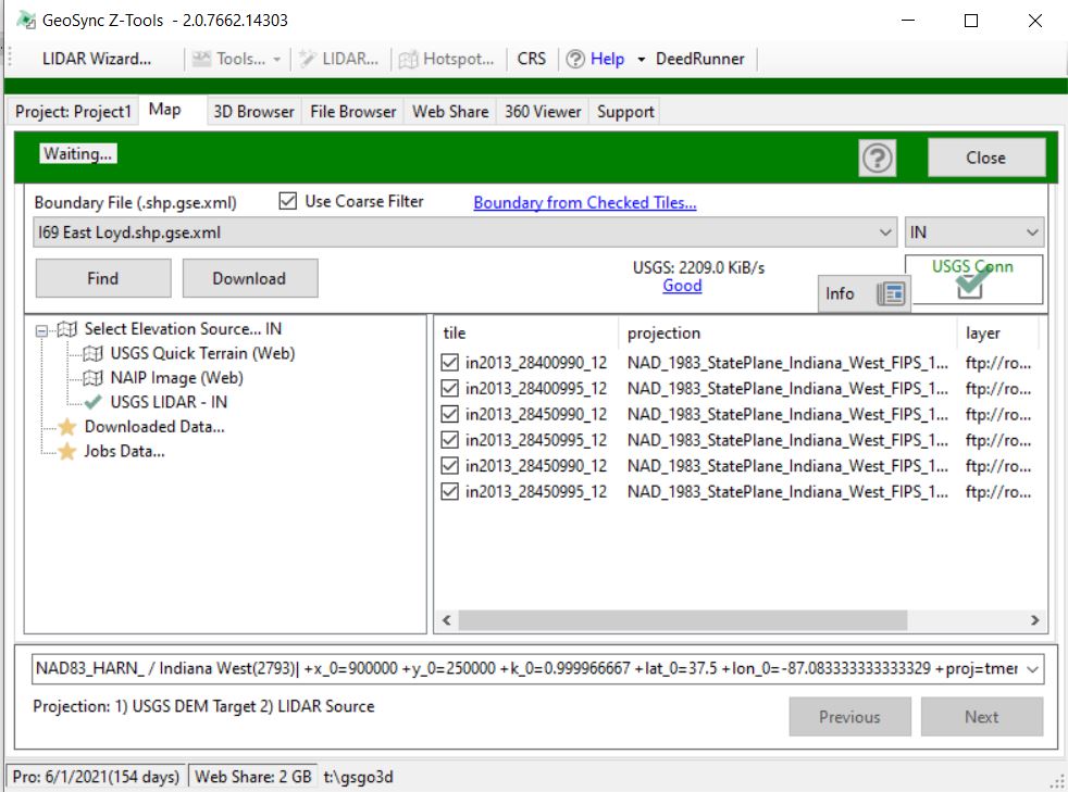
- All other items: The application will perform a detailed search and return a list of available tiles for download. The list will include the tile name, tile map projection, and USGS project (date) of the tile. Check the tiles you want to download and click the download button. The tiles will be downloaded to your project tile_downloads folder.
-
Set the Map Projection to Match the Downloaded Tiles – if the correct projection is not in the dropdown list then use the CRS tool on the Tool Strip to search
-
Select a Downloaded Data Source – from the tree list under Downloaded Data The selected folder will return a list of available downloaded LIDAR tiles. Check the tiles you want to use for clipping and processing.
-
Click the Next button to continue
-
Processing Options -
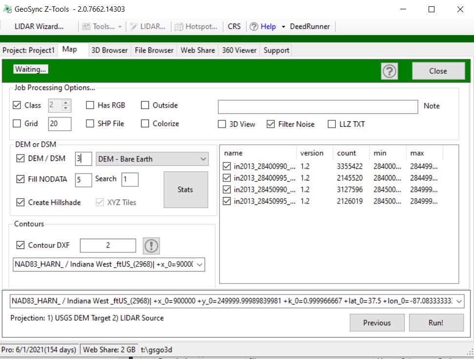
- Job Processing Standard options
- Class – Check to filter only the points classified as ground points
- Grid – grid points based on the value specified to produce an output with points grid spacing
- Has RGB – check if source point cloud has RGB attributes and you want to preserve these attributes in the final output
- SHP File – check if you want to generate a SHP file output of point cloud points
- Outside – check if you want to clip “outside” the boundary layer instead of the default “inside” the boundary layer
- Colorize – check to colorize the clipped point cloud using USGS NAIP imagery
- Note - enter a descriptive note for this job
- Publish 3D View – publish a 3D view of the clipped point cloud data and display
- DEM or DSM – Digital terrain options
- DEM/DSM – check if you want to create a digital terrain output in TIF format. This is option is necessary to generate hillshade and / or contours.
- Set the output width / height map distance for the generated TIF file. This size value must be greater than or equal to point cloud xy plane density.
- Select from the dropdown to set whether to use bare earth, mean or max elevations
- Fill NODATA – check if you want to fill holes in the digital terrain output by averaging pixel elevations. Set the maximum NODATA pixel radius from pixels with elevation data for averaging. If the pixel size is 1 foot and fill NODATA value is 5 then averaging will extend about 5 feet beyond pixels with data to fill holes.
- Search – multiplier times the DEM/DSM size used in creating the DEM/DSM cell elevation
- Stats button – provides information on the expected size in pixels of the DEM/DSM TIF output
- Create Hillshade – checking this option generates a hillshade TIF from the DEM/DSM TIF and automatically builds an XYZ Tile Layer of the hillshade and a local DEM/DSM file for use in the Project Map. Local DEM/DSM is exported in ASC format.
- Contour options
- Check the DXF Contour option to output contours. Enter the contour interval in map units. Contours will be generated in SHP and DXF format.
- Select the output map projection for the DXF Contours. SHP format contours do not utilize this option when created.
- Job Processing Standard options
-
Click the Run! button to begin processing the data. A processing log is displayed reporting on the steps. Once processing is complete the output files will be automatically copied to a Jobs folder.
-
Use File Browser to open the Job Folder or Click Previous and Change Options to Run again and generate new Job outputs